Matlab R2014a on Mac Maverick Retina Display

Hi guys,

• I think you have also encountered that the Matlab GUI is blurry. 
• The reason for this is that previous versions of Matlab like R2013b (and R2014a) includes a Java runtime (JRE) on the package itself, which however does not support the new features like Retina displays.
• As a workaround, you can install the latest JRE and make Matlab point to this JRE.
• This is how it is done. Credit should go to original contributors; I am just putting the links here.
• Install latest JRE from link (you can choose jre-7u71-macosx-x64.dmg); may be you want to restart the machine.
• Create an AppleScript with the following script and save it as app. Note that all the code needs to be in one line.

do shell script "export MATLAB_JAVA=\"/Library/Internet Plug-Ins/JavaAppletPlugin.plugin/Contents/Home\"" & "; export MATLAB_USE_USERWORK=1" & ";/Applications/MATLAB_R2014a.app/bin/matlab -desktop &> /dev/null &"

• To create an AppleScript: Finder->Applications and find for AppleScript Editor (find within applications; not "This Mac") and paste the above script
• Save it as an app.
• If you would like to change its icon, 
• select app in Finder and open app directory through “Show Package Contents”
• go to Contents/Resources and copy/paste the new icon (.icns file) onto applet.icns (you can find Matlab icons from Matlab application folder itself)
• the above steps themselves do not work usually, so do the following as well.
• select the app, again in Finder and this time, click on “Get Info”
• select the app icon at the top - a blue outline will appear
• copy the icon (.icns file) onto this outlined icon (command-v)
• now, check the .app directory using a terminal - “ls -la”
• the “Icon?” file should be there
• delete this file - “rm Icon^M”
• immediately, the app should have the copied icon beside it in the Finder

Credit should go to

• Florian @ link
• Asanga @ link

Cheers!

Remove Pyramid Grid from ODE Drawstuff

Hi,

Here is how it is done.

• In the ode source find drawstuff.cpp
• In that you will find the call to the method drawPyramidGrid();
• comment this out
• Next, run the following in the source folder

$ ./configure --enable-double-precision --enable-shared
         $ make
         $ make install

• To copy .h files and libraries to /usr/local/include and /usr/local/lib: 

$ sudo make install
$ sudo cp -p drawstuff/src/.libs/libdrawstuff.a /usr/local/lib/
$ sudo cp -p drawstuff/src/libdrawstuff.la /usr/local/lib/
$ sudo cp -rp include/drawstuff /usr/local/include/
$ sudo cp -rp drawstuff/textures /usr/local/include/drawstuff/


That's it
Cheers!

DC Motor Torque, Speed

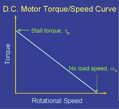
There is a torque-speed curve for motors, which looks like:

[reference: link]

• This curve has been drawn for constant voltage and changing load.
  

• First things first. There is no need to confuse the word “torque” related to a motor.

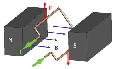
  If we recall that when a current carrying conductor in a magnetic field is subjected to a force and it is this force that creates the torque to rotate the rotor (conductor), it is this torque we are still talking about.
  [reference: link]

  • If there is a load attached to the rotor it wont affect the torque generated by the motor as it only depends on the current, the field, number of turns and the area of the coil.
    T = BINA Cosθ
    

• It is important to note that the above curve has not been drawn for transients of motor speed; it is drawn for the final stabilized speed ω of the motor.

• We discuss the transients of motor speed in order to understand what is going on but will draw the stabilized speed ω in the curve versus the torque.

• Let's say we have some fixed load attached to the motor and the applied voltage is constant.

• Now there is one thing we should remember. That is the existence of electrical torque and mechanical torque.

  • We already know what electrical torque is.

  • Mechanical torque is the usual force x distance in relation to the load.

  • That is the mechanical torque we need to turn the input shaft of the load.

  • When the motor is running in steady state, the armature current is constant, and the electrical torque is equal and opposite of the mechanical torque or load torque. 

  • When the motor is decelerating, the motor torque is less than the load torque. Conversely, when a motor is accelerating, the motor torque is higher than the load torque.
      

  • so, it is the resultant torque, τm - τl = τ, that will account for the acceleration of the load. 

  • This is somewhat like friction when we apply a force to a box or something.
    

• At the beginning, ω=0 and CEMF (counter electro motive force or back emf), which is proportional to ω, will be zero.

• Without any CEMF and small resistance of the coil, a huge current will be drawn from the DC source.

• This will result in large torque τm; torque is proportional to current (or current2 in series DC motor).

• τm - τl = τ will be large and ω will gradually increase.

• When ω increases, however, there will be CEMF building up, which will reduce the applied voltage to the current coil.
  VDC – CEMF = v (VDC const.)

• When v drops → the current drops → τm drops → τm - τl = τ drops

• There will be, however, a torque and still there will be acceleration. What is happening is that this acceleration is gradually decreasing.

• Finally,  τm = τl  and there wont be any resultant torque. 

• As a result, ω will stabilize → CEMF will stabilize → VDC – CEMF = v will stabilize → current i will stabilize.

• Now we have a point in curve. (τm, ω)

Reduce load (or load torque)

• Now, we reduce the load. This means the mechanical torque required to turn the load τl will be reduced.

• And we start everything from the beginning  ω=0

• Now τm - τl = τ will be large. (τl has become smaller)

• As a result, the acceleration of motor will be high. So, ω will attain higher values than the previous case.

• Again CEMF will come into play. And, τm will start to decrease and will eventually equal τl which is smaller than the previous case.

• As a result, ω will stabilize (at a higher value) → CEMF will stabilize → VDC – CEMF = v will stabilize → current i will stabilize.

• Now we have another point in the curve. This time the torque will be lesser and ω will be higher, than the previous case.
  

• So we saw that when the load (or load torque) decreases we need a small τm at stability. That is we needed little current. That is we needed VDC – CEMF = v to be small. This is achieved by higher CEMF, which is achieved by higher ω. 

• For a huge load (or load torque), τm  will not be sufficient to turn the motor. Therefore,  ω=0 and there wont be any CEMF. Thus, i max → τmax 

• Actually, this is kind of equal to the case of initial instance of a regular load, too. The only difference is the starting torque is enough to drive the load in this case.

Increase speed

• For a given load we saw that ω stabilizes after its initial transients.

• So, how can we increase the speed for a given load (e.g. fan)?

• To increase speed we need more torque τm.

• That is we need more current.

• The only way we can do that is by increasing the voltage.

• When the voltage is increased, we have more current and we will have a resultant torque.

• This will increase the speed ω from its current value.

• Again CEMF will come into play and, the resultant voltage will be reduced.

• When v drops → the current drops → τm drops → τm - τl = τ drops.

• Finally,  τm = τl  and there wont be any resultant torque. 

• As a result, ω will stabilize → CEMF will stabilize → VDC – CEMF = v will stabilize → current i will stabilize.

• Note that in this case ω has stabilized at a higher value than previous.  

Runaway

• Let's say we want to control current/torque in a motor.

• Assume that with a given load, the motor was drawing, say 100mA, turning at a speed of 1000rpm  and everything is steady.

• Say we wanted to control current at 200mA.

• And we increase the voltage.

• So the current increases →  ω increases → CEMF increases → current starts to decrease.

• That is we need higher voltage to maintain the current at the new set value.

• Higher voltage → higher ω → higher CEMF → higher applied voltage needed → higher ω …

• As a result, the motor speed runs away up to the maximum speed that is possible with the given supply voltage.

• Such a runaway condition can occur unless it is limited by a higher-level control loop (velocity or position control), a mechanical stop (e.g. stopping by hand) or an additional safety speed limitation.

cheers!

et al. in Latex References

Hi guys,

I use a separate .bib file for including references in my LaTex documents.
i.e.
\bibliography{bib/mybib}
\bibliographystyle{IEEEtrans}

where bib is a folder and mybib.bib is the bibliography file. It has entries in the following format.

@article{dissanayake2001solution,
  title={A solution to the simultaneous localization and map building (SLAM) problem},
  author={Dissanayake, MWM Gamini and Newman, Paul and Clark, Steve and Durrant-Whyte, Hugh F and Csorba, Michael},
  journal={Robotics and Automation, IEEE Transactions on},
  volume={17},
  number={3},
  pages={229--241},
  year={2001},
  publisher={IEEE}
}

Now, if you are running out of space you can make the author list small by using et al. keyword. To use that just type "and others" in the authors sub-entry like this.

@article{dissanayake2001solution,
  title={A solution to the simultaneous localization and map building (SLAM) problem},
  author={Dissanayake, MWM Gamini and others},
  journal={Robotics and Automation, IEEE Transactions on},
  volume={17},
  number={3},
  pages={229--241},
  year={2001},
  publisher={IEEE}
}

By the way, you can export entries to BibTex from Google Scholar. Go to settings in Google scholar and in Bibliography manager "Show links to import citations into" choose BibTex.

That's it.


Cheers!!!

Writing Japanese using pLatex in Mac

This is how it is done!

First of all, the credit should go to Link and I am just copying from there.

• Install Macports from here; follow any additional steps stated by them.
• After installing Macports, type the following on the terminal

sudo port install pTeX +hiragino +otf +utf8 +motif +macosx

• Install TeXShop if you do not already have it.
• Open preferences in TeXShop and select "Set Default Values". In the drop down menu, choose Legacy pTeX (Shift JIS)
• Save your tex file using Japanese SJIS encoding.
• Press "Typeset" to build your file
• If things are not working try the following.
• modify the file “/Users/<your account>/Library/TeXShop/bin/platex2pdf-euc” to change path to “opt” instead of “usr”. That is 

from [export PATH=$PATH:/usr/local/bin:/usr/local/teTeX/bin] 

to [export PATH=$PATH:/opt/local/bin:/usr/local/teTeX/bin]

• If fontspec is needed:

sudo tlmgr update –self
sudo tlmgr install fontspec

• Here is a sample code

%\documentclass[twocolumn,11pt]{jarticle} %In case two column layout

\documentclass[a4j]{jarticle}

\usepackage{graphicx} %for including graphics

\usepackage{nidanfloat}

\usepackage{url}

\title{タイトル}

\author{ 僕の名前 }

\date{2010年}

\renewcommand{¥refname}{References}

\begin{document}

\maketitle

\section{テスト}

これはテストです。

\end{document}